Spatial Pattern Analyses
Problem
We are tasked to work through several exercises to Analyze patterns and identify clustering areas of incident calls occurring in the Dallas as well as the city of Orleander. Focused on the 2nd Battalion Fire Department and census data from those areas.
Analysis procedures
Strategies
The data was provided for the GIS Tutorials via four file geodatabases. Census.gdb, City of Ft Worth.gdb, City of Oleander.gdb and Libray.gdb. I used ArcCatalog to view the data structures and identify key Feature Datasets, Classes, and Layers. I then used ArcMap to open the appropriate map .mxd files associated with exercises 8.1, 8.2. 8.3, 8.4, 9.1. 9.2. Each labeled Tutorial X.X.mxd in direct correlation to the tutorial/exercise being worked. The six exercises focused on the specific tools in each beginning with 8.1, Analyzing patterns using the Average Nearest Neighbor and z-score and confidence level analysis. 8.2 focused on the high/low clustering (Getis-Ord General G tool) and investigated threshold distances in comparison with the z-score statistic to determine probability of the Null Hypothesis. 8.3 utilized the multi-distance spatial cluster analysis (Ripley's L function) which measures the distance between points to determine clustering and utilize several tools to create graphs and add the graphs to the map for future interpretation. 8.4 utilized a grid overlay which was joined to the data to create a grid of the points of interest. This new grid was then use with the Spatial Auto Correlation tool to determine the highest z-score based on a series of distances to confirm/reject the null hypothesis. 9.1 we used the Cluster and Outlier Analysis tool to determine if the high z-scores were because of high values or not associated with the clusters. Finally in 9.2 we use the Hot spot analysis tool to determine clusters of high incidents/income areas and low incident/income areas.
Methods
Exercise 8.1
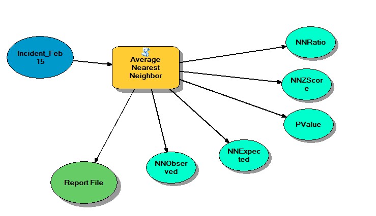
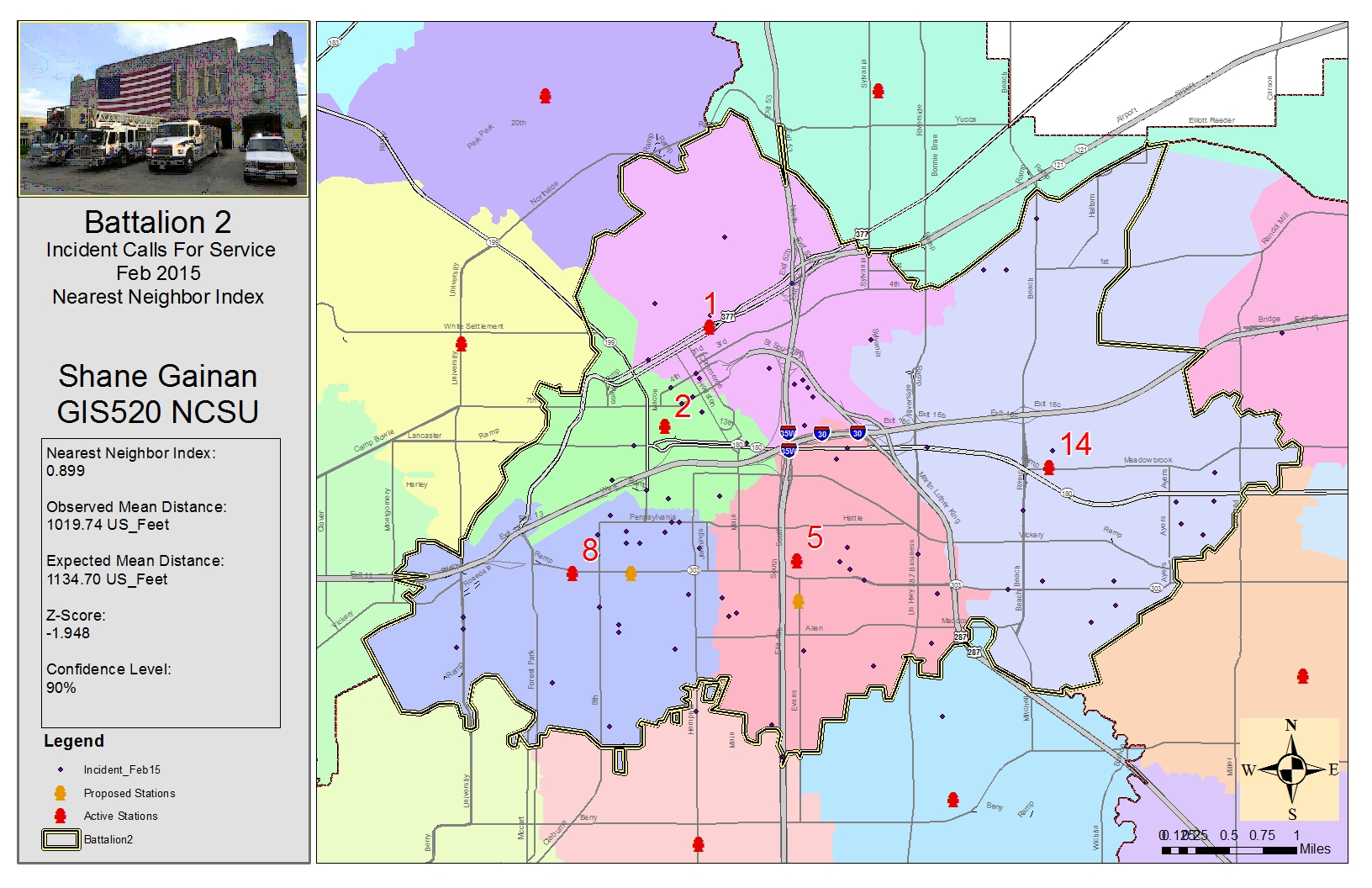
After opening the Tutorial 8-1.mxd I created a definition query within the properties of the incident_Feb15 layer to ensure the range of incident types is equal to and between 700-745. ([inci-type] >= ‘700’ AND [inci-type] <=’745’). And then run the Average Nearest Neighbor tool by selecting the Input Feature Class: Incident_Feb 15 and defining the Area: 520175356, the Area is based on the Battalion_2 Feature Class and Area in which that battalion is responsible for. We want to create a report so we selected the Generate Report Box and ran the tool.
The results can be found in the results window by double clicking the HTML report file to open the graphical display and record the results on the map. The results give us the Observed Mean Distance, Expected Mean Distance, Nearest Neighbor Ratio, and Z-Score. To interpret these results and determine if the incident was random or not you use the Nearest Neighbor Ratio, our results indicated 0.899 thus indicating that it is probably not random that the incidents occurred in those areas with a 90% confidence level based of our z-score of -1.948.
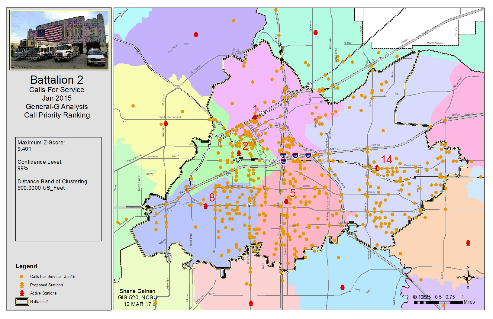
Exercise 8.2
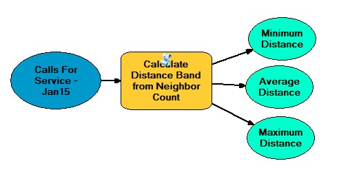
After opening the Tutorial 8-2E.mxd calculate
distance band from neighbor count (spatial statistics) to determine the
appropriate distance to begin the High/Low Clustering (Getis-Ord General
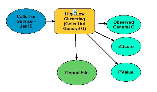
G) tool. In this case it was around 1100 feet. In this case we began the
calculations at 700 feet incrementing up to 1200 feet in search of the
highest z-score, which was found at approximately 900 feet. This showed
the peak value at which clustering was the most prevalent.
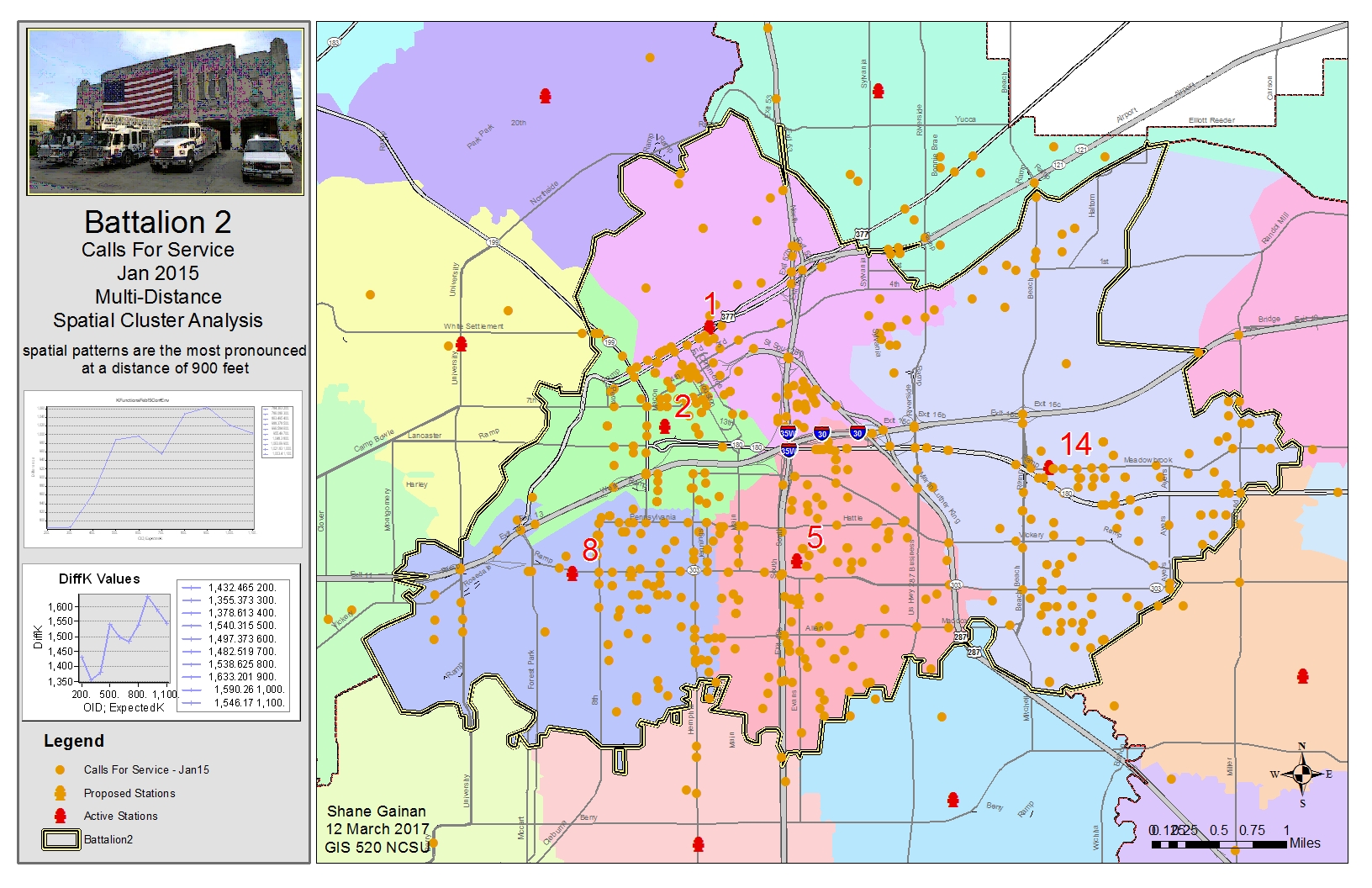
Exercise 8.3
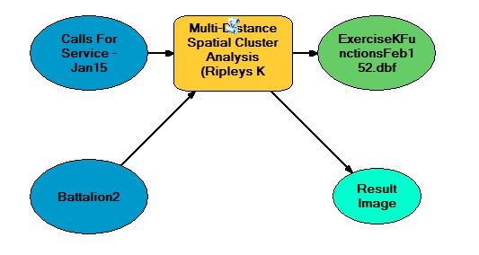
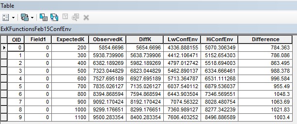
After opening the Tutorial 8-3E.mxd I opened the multi-distance spatial cluster analysis (Ripley's k function) (spatial statistics) after setting the parameters as in the tutorial we first produced the K Function which the results were stored in our KFunctionFeb15 table. We then made a graph from this table to add to the map by selecting the Create Graph utility in the menu. Ensuring the graph type was a vertical line, Y field set to DiffK, and the X label field set to ExpectedK and right clicking to add that to the map. We than reran the Multi-Distance Spatial Cluster Analysis tool using a confidence envelope of 99 Permutations saving the results into a table call KFunctionFeb15ConfEnv. Within this table depicted at the end of this document we added a Difference field of the obeservedK subtracting HiConfEnv and made a graph from the table. The Graph was set to Difference as the Y field and Expected K as the x label field and add that image to the map.
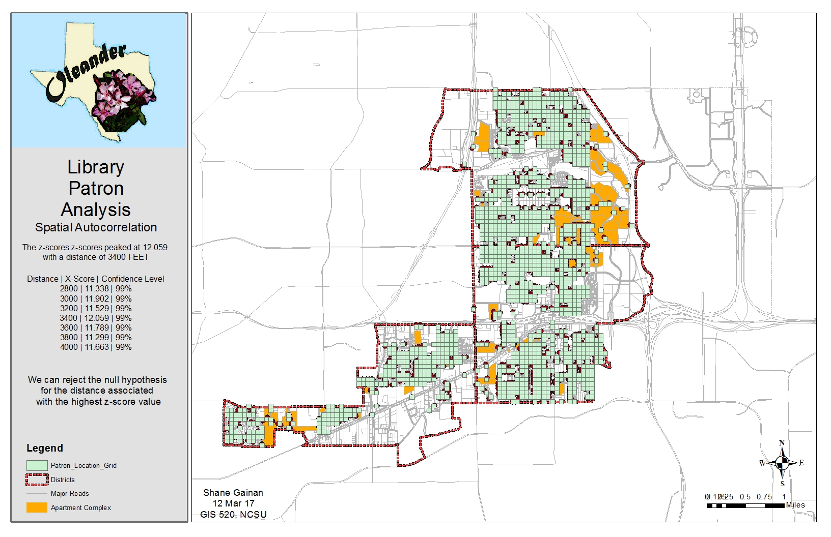
Exercise 8.4
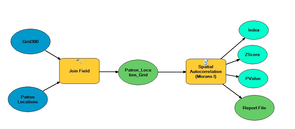
After opening the Tutorial 8-4E.mxd I created a join of tables of the Grid300 and the Patron Locations to identify the grid of were these intersected. I then created a definition query within the newly joined feature class to only show Count_ > 0, this eliminated the grids which did not have an intersection of the patron location.
After completed the join and identifying the correct locations I ran the Spatial Autocorrelation (Global Moran’s i) with distances bands of varying distance beginning with 2800 and incremental by 200 until I captured approximately seven iterations. This gave me a Z-Score for each distance and highlighted the highest Z-Score of 12.059 this gave me the highest probability that the clustering of locations was not by chance at a Distance band of 3400 feet. Thus rejecting the Null Hypothesis that the clustering was by random chance.
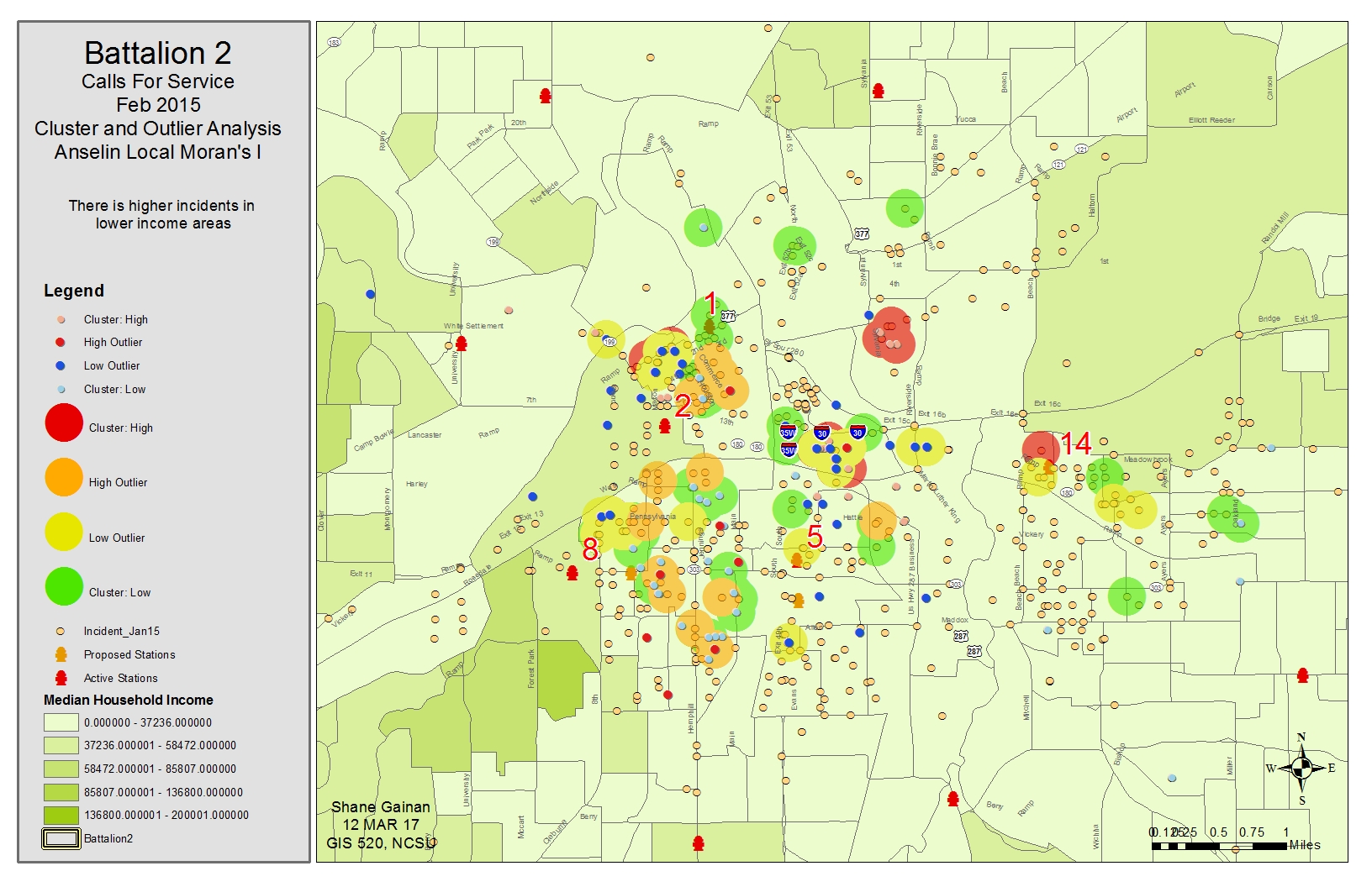
Exercise 9.1
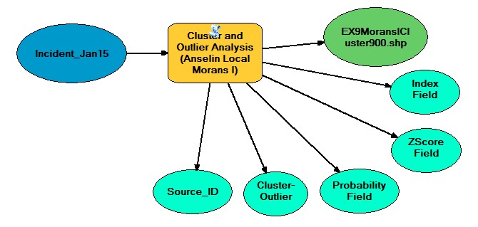
After opening the Tutorial 9-1E.mxd we ran the Cluster and outlier analysis (anselin local moran's i) (spatial statistics) which in turn created an Output Feature Class: IncidentMoransICluster.shp. I then created a copy of the new layer and named it ClusterTypes and changed the symbology to unique values and added those values of HH, HL, LH, LL as the values. I then re-ran the Cluster and Outlier analysis tool using the fixed distance band of 900 feet. Once completed the IncidentMoransICluster900.shp was created and I changed they symbology as previously and added the values to depict on the map. This gave me values that showed clustering (Positive) and dispersion (negative) of the incidents for comparison.
Exercise 9.2
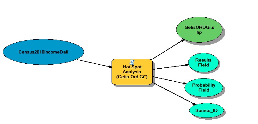
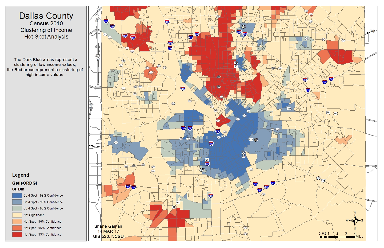
After opening the Tutorial 9-2E.mxd I ran the hot spot analysis (getis-ord gi*) (spatial statistics) Tool. Within this tool I sued the Input feature class Census2010IncomeDall and located the input field of P053001. After running the tool with a distance band of 5280 feet an output feature class named GetisORDGi.shp was created.
This tool enabled me to see the clustering results based on another field, in this case the household income. Showing high income and low income cluster areas. It produced a very defined map of the distinct areas.
Process diagram / workflow diagram
Average Nearest Neighbor Tool
Calculate Distance Band from Neighbor Count
High Low Clustering Tool
Multi-Distance Spatial Cluster Analysis Tool
Use Join and Spatial Autocorrelation Tools
Cluster and Outlier Analysis Tool
Hot Spot Analysis Tool
Results
Exercise 8.1
Exercise 8.2
Exercise 8.3
Exercise 8.4
Exercise 9.1
Exercise 9.2
Application and Reflection
In reflection of the exercise and the future application of it I can see many different uses. In the examples we say incident calls to a particular EMS and Fire Department.
Problem description
This type of analysis could be used in a military application as well. Due to my experience in the Military I think if you had the data for attacks in an Area of Operation on friendly forces you could utilize these tools to determine if they are clustered in certain areas through statistical analysis and determine if the occurrences are random or not to aid in planning military operations in those areas. You could possibly save lives by knowing that the probability of an attack happening in a certain area is more likely going to happen or if it is a random chance it will happen.
Data needed
The data in needed for my analysis would come from military classified systems documenting events and theater maps
Analysis procedures
Using one or a combination of all the tools outlined above I would calculate the appropriate z-score then determine the probability of that hypothesis being true or false. In my thoughts I would use a combination of the tools above to determine the probability that an attack was random or possibly something more predictable based on enemy activity in the area.